Generate Code and Export Fits to the Workspace

Generating Code from the Curve Fitting App

You can generate and use MATLAB^® code from an interactive session in the Curve Fitting app. In this way, you can transform your interactive analysis into reusable functions for batch processing of multiple data sets. You can use the generated file without modification, or you can edit and customize the file as needed.

To generate code for all fits and plots in your Curve Fitting app session follow these steps:

Select File > Generate Code.
The Curve Fitting app generates code from your session and displays the file in the MATLAB Editor. The file includes all fits and plots in your current session. The file captures the following information:
- Names of fits and their variables
- Fit settings and options
- Plots
- Curve and surface fitting objects and methods used to create the fits:
  - A cell-array of cfit or sfit objects representing the fits
  - A structure array with goodness-of fit information.
Save the file.

To recreate your fits and plots, call the file from the command line with your original data as input arguments. You also can call the file with new data.

For example, enter:

[fitresult, gof] = myFileName(a, b, c)

where a, b, and c are your variable names, and myFileName is the file name.

Calling the file from the command line does not recreate your Curve Fitting app and session. When you call the file, you get the same plots you had in your Curve Fitting app session in standard MATLAB figure windows. There is one window for each fit. For example, if your fit in the Curve Fitting app session displayed main, residual and contour plots, all three plots appear in a single figure window.

Curve Fitting Functions

The curve and surface fit objects (cfit and sfit) store the results from a fitting operation, making it easy to plot and analyze fits at the command line.

To learn about available functions for working with fits, see Curve and Surface Fitting.

Exporting a Fit to the Workspace

To export a fit to the MATLAB workspace, follow these steps:

Select a fit and save it to the MATLAB workspace using one of these methods:
- Right-click the fit listed in the Table of Fits and select Save myfitname to Workspace
- Select a fit figure in the Curve Fitting app and select Fit > Save to Workspace.
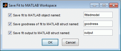
The Save Fit to MATLAB Workspace dialog box opens.
Edit the names as appropriate. If you previously exported fits, the toolbox automatically adds a numbered suffix to the default names so there is no danger of overwriting them.
Choose which options you want to export by selecting the check boxes. Check box options are as follows:
- Save fit to MATLAB object named fittedmodel — This option creates a cfit or sfit object, that encapsulates the result of fitting a curve or surface to data. You can examine the fit coefficients at the command line, for example:
```
 fittedmodel
    Linear model Poly22:
       fittedmodel1(x,y) = p00 + p10*x + p01*y + p20*x^2...
                           + p11*x*y + p02*y^2
     Coefficients (with 95% confidence bounds):
       p00 =       302.1  (247.3, 356.8)
       p10 =       -1395  (-1751, -1039)
       p01 =     0.03525  (0.01899, 0.05151)
       p20 =        1696  (1099, 2293)
       p11 =     -0.1119  (-0.1624, -0.06134)
       p02 =   2.36e-006  (-8.72e-007, 5.593e-006)
```
  You also can treat the cfit or sfit object as a function to make predictions or evaluate the fit at values of X (or X and Y). See the cfit and sfit reference page.
- Save goodness of fit to MATLAB struct named goodness — This option creates a structure array that contains statistical information about the fit, for example:
```
goodness = 
           sse: 0.0234
       rsquare: 0.9369
           dfe: 128
    adjrsquare: 0.9345
          rmse: 0.0135
```
- Save fit output to MATLAB struct named output — This option creates a structure array that contains information such as numbers of observations and parameters, residuals, and so on. For example:
```
output = 
        numobs: 134
      numparam: 6
     residuals: [134x1 double]
      Jacobian: [134x6 double]
      exitflag: 1
     algorithm: 'QR factorization and solve'
    iterations: 1
```
  Note
  Goodness of fit and Output arrays are outputs of the fit function. See the fit reference page.
Click OK to save the fit options to the workspace.

After you save your fit to the workspace, you can use fit postprocessing functions. For an example, see Analyzing Your Best Fit in the Workspace. For more information and a list of functions, see Fit Postprocessing.

Documentation